




概述
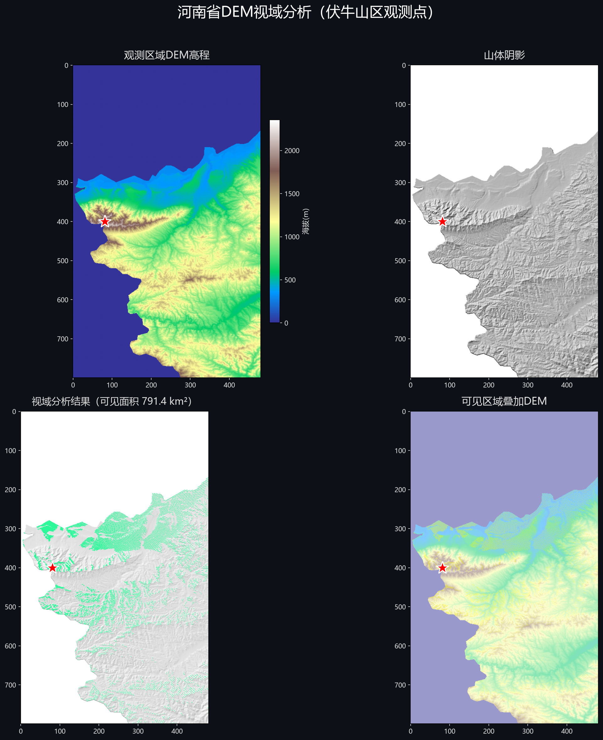
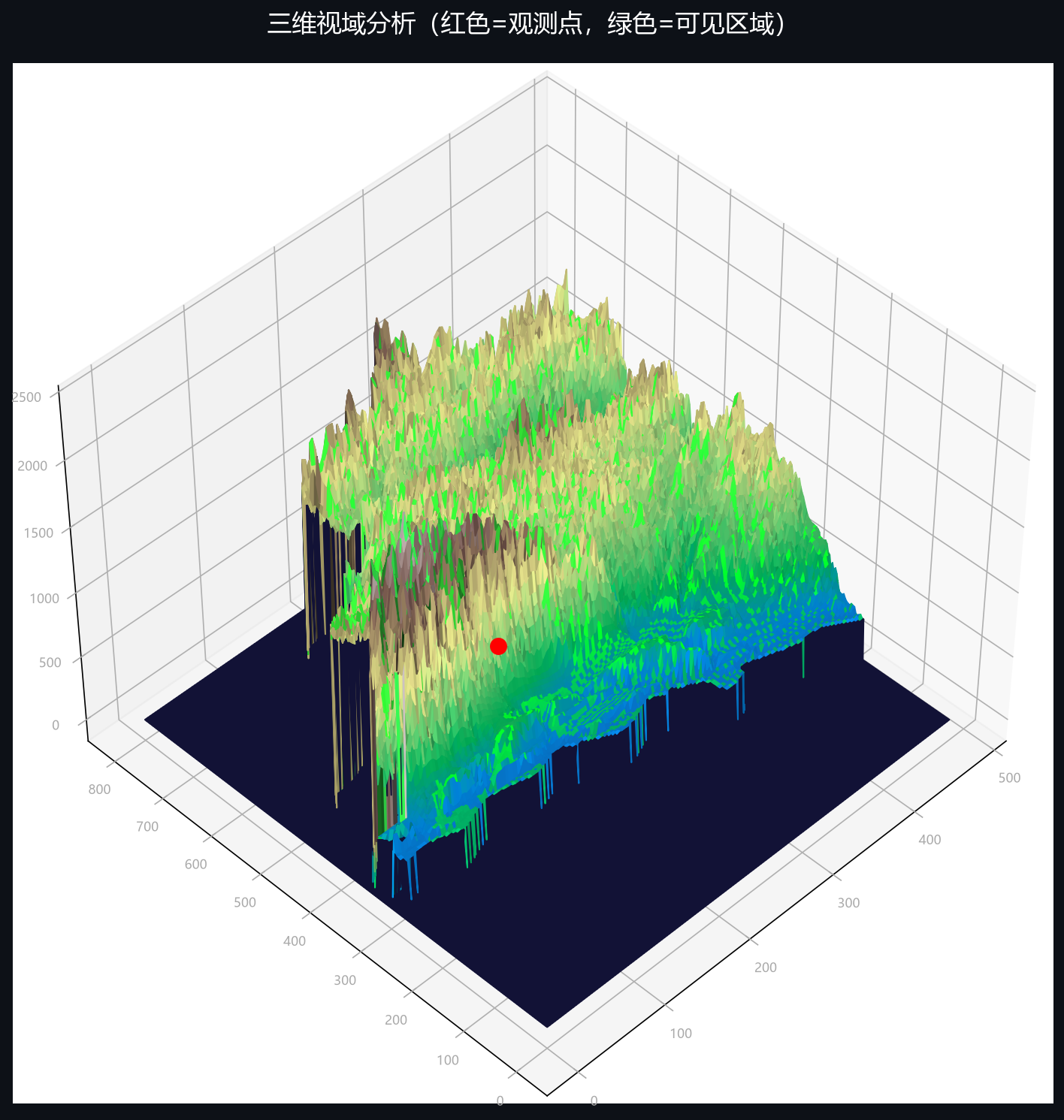
视域分析(Viewshed)是DEM最具实用价值的应用之一——计算在指定观测点观察时,地表的可见/遮挡区域分布。本文从视线追踪算法原理到代码实现,完整讲解单点视域、累积视域和最优选址。
数据基础:ASTER GDEM V003,30m分辨率,WGS84(EPSG:4326),int16,NoData=-9999。全国34省已裁切,覆盖N18°~N53°、E73°~E134°。
1. 原理
1.1 视线追踪(Line of Sight)
核心算法是视线追踪。设观测点O、目标点T,沿O→T方向的中间像素序列为 P_1, P_2, …, P_n。
视线上 P_i 处的高程(线性插值):
los_h(P_i) = h_O + (h_T - h_O) × |O→P_i| / |O→T|
其中 h_O = DEM[O] + 观测高度,h_T = DEM[T] + 目标高度。
判断规则:如果存在 i ∈ {1, …, n-1} 使得 DEM[P_i] > los_h(P_i),则T不可见。
1.2 计算复杂度
省级DEM(~5000×5000),GDAL单点视域约30秒~2分钟。
1.3 地球曲率校正
搜索半径>10km时需考虑地球曲率。距观测点d处,目标点相对切平面的下降量:
Δh = d² / (2R) ≈ d² / 12742000 (R≈6371km)
标准大气折射使视线弯曲向下,等效地球半径增大约1/6,实际校正系数为0.85714(=1/1.1667)。
2. 关键参数
2.1 参数清单
2.2 观测高度与视域关系
高度越高视域越大,但边际效益递减。山区30m DEM上典型规律:
3. Python实现
3.1 GDAL命令行(推荐)
# 基本视域
gdaldem viewshed dem.tif viewshed.tif \
    -ox 114.5 -oy 30.5 \   # 观测点经纬度
    -oz 1.7 \               # 观测高度(m)
    -md 10000               # 最大搜索半径(m)

# 通信基站(30m高,15km半径,含曲率校正)
gdaldem viewshed dem.tif vs_celltower.tif \
    -ox 114.5 -oy 30.5 \
    -oz 30 -md 15000 \
    -cc 0.85714

# 瞭望塔(15m高,12km半径)
gdaldem viewshed dem.tif vs_watchtower.tif \
    -ox 114.5 -oy 30.5 \
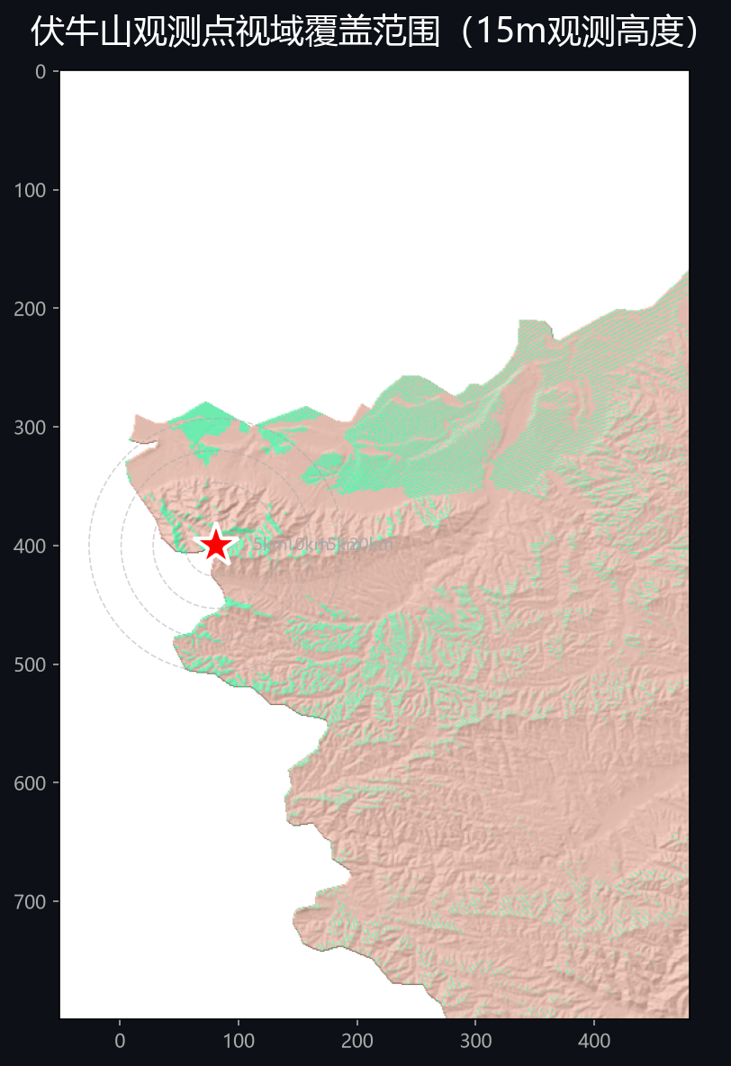
    -oz 15 -md 12000 \
    -cc 0.85714
3.2 WhiteboxTools
from whitebox import WhiteboxTools

wbt = WhiteboxTools()
wbt.set_workdir("/path/to/data/")

wbt.viewshed(
    "dem.tif",
    "viewshed.tif",
    "--viewpoint 2500,1800",   # 像素坐标(row,col)
    max_dist=10000              # 最大距离(m)
)
3.3 numpy手写版(原理理解用)
import numpy as np
import rasterio

def viewshed_numpy(dem_path, vp_row, vp_col, obs_height=1.7,
                   max_dist_m=10000, target_height=0.0,
                   curvature=True):
    """
    视域分析(numpy手写版)

    参数:
        dem_path: DEM文件路径
        vp_row, vp_col: 观测点像素坐标
        obs_height: 观测高度(m)
        max_dist_m: 最大搜索半径(m)
        target_height: 目标高度(m)
        curvature: 是否进行地球曲率校正

    返回:
        visibility: 可见性矩阵(1=可见, 0=不可见)
    """
    with rasterio.open(dem_path) as src:
        dem = src.read(1).astype(np.float64)
        nodata = src.nodata
        if nodata is not None:
            dem[dem == nodata] = -9999
        cellsize_m = abs(src.res[0]) * 111320.0  # 度→米

    rows, cols = dem.shape
    max_pixels = int(max_dist_m / cellsize_m)

    # 观测点高程 + 观测高度
    h_obs = dem[vp_row, vp_col] + obs_height
    R_eff = 6371000.0 * 1.1667  # 大气折射等效地球半径

    visible = np.zeros_like(dem, dtype=np.uint8)
    visible[vp_row, vp_col] = 1

    r_min = max(0, vp_row - max_pixels)
    r_max = min(rows, vp_row + max_pixels + 1)
    c_min = max(0, vp_col - max_pixels)
    c_max = min(cols, vp_col + max_pixels + 1)

    for r in range(r_min, r_max):
        for c in range(c_min, c_max):
            if r == vp_row and c == vp_col:
                continue

            # 距离计算
            dr = r - vp_row
            dc = c - vp_col
            dist_m = np.sqrt(dr**2 + dc**2) * cellsize_m
            if dist_m > max_dist_m:
                continue

            h_target = dem[r, c] + target_height

            # 曲率校正:目标点下降量
            if curvature:
                h_target -= dist_m**2 / (2 * R_eff)

            # 生成视线上的采样点
            n_samples = max(int(dist_m / cellsize_m), 2)
            line_r = np.linspace(vp_row, r, n_samples + 1).astype(int)
            line_c = np.linspace(vp_col, c, n_samples + 1).astype(int)

            # 视线高程(线性插值)
            t = np.linspace(0, 1, n_samples + 1)
            los_h = h_obs + (h_target - h_obs) * t

            # 曲率校正:视线上每点的下降量
            if curvature:
                dist_along = t * dist_m
                los_h -= dist_along**2 / (2 * R_eff)

            # 检查遮挡
            terrain_h = dem[line_r, line_c]
            # 排除端点(起点和终点本身)
            blocked = np.any(terrain_h[1:-1] > los_h[1:-1] + 0.01)

            visible[r, c] = 0 if blocked else 1

    return visible


def save_viewshed(visible, ref_path, out_path):
    with rasterio.open(ref_path) as src:
        profile = src.profile.copy()
    profile.update(dtype='uint8', nodata=255)
    with rasterio.open(out_path, 'w', **profile) as dst:
        dst.write(visible.astype(np.uint8), 1)
注意:numpy版O(N^1.5),仅用于理解。生产环境使用GDAL或WhiteboxTools。
3.4 可视化
import matplotlib.pyplot as plt
from matplotlib.colors import ListedColormap

def plot_viewshed(dem_path, viewshed_path, vp_row, vp_col):
    fig, axes = plt.subplots(1, 3, figsize=(20, 7))

    with rasterio.open(dem_path) as src:
        dem = src.read(1).astype(float)
        dem[dem == src.nodata] = np.nan
    with rasterio.open(viewshed_path) as src:
        vis = src.read(1)

    # DEM
    ax = axes[0]
    im = ax.imshow(dem, cmap='terrain')
    ax.plot(vp_col, vp_row, 'rv', markersize=14, zorder=5)
    ax.set_title('DEM高程', fontsize=14, fontweight='bold')
    plt.colorbar(im, ax=ax, shrink=0.7, label='m')

    # 视域二值图
    ax = axes[1]
    cmap = ListedColormap(['#bdc3c7', '#27ae60'])
    ax.imshow(vis, cmap=cmap, vmin=0, vmax=1)
    ax.plot(vp_col, vp_row, 'rv', markersize=14, zorder=5)
    ax.set_title('视域(绿=可见 灰=遮挡)', fontsize=14, fontweight='bold')

    # 叠加(DEM半透明 + 视域高亮)
    ax = axes[2]
    ax.imshow(dem, cmap='gray')
    masked = np.ma.masked_where(vis == 0, vis)
    ax.imshow(masked, cmap=ListedColormap(['#2ecc71']), alpha=0.5)
    ax.plot(vp_col, vp_row, 'r^', markersize=14, zorder=5)
    ax.set_title('叠加效果', fontsize=14, fontweight='bold')

    plt.tight_layout()
    plt.savefig('viewshed_result.png', dpi=150, bbox_inches='tight')
    plt.show()
4. 累积视域与最优选址
4.1 累积视域(Cumulative Viewshed)
def cumulative_viewshed(dem_path, viewpoints, out_path,
                        max_dist=10000, obs_h=15):
    """多观测点累积视域"""
    wbt = WhiteboxTools()
    cumul = None

    for i, (r, c) in enumerate(viewpoints):
        tmp = f"tmp_vs_{i}.tif"
        wbt.viewshed(dem_path, tmp, f"--viewpoint {r},{c}",
                     max_dist=max_dist)
        with rasterio.open(tmp) as src:
            v = src.read(1).astype(np.int16)
        cumul = v if cumul is None else cumul + v

    # 保存
    with rasterio.open(dem_path) as src:
        profile = src.profile.copy()
    profile.update(dtype='int16', nodata=-1)
    with rasterio.open(out_path, 'w', **profile) as dst:
        dst.write(cumul.astype('int16'), 1)

    # 统计
    total = cumul.size
    covered = (cumul > 0).sum()
    multi = (cumul >= 2).sum()
    print(f"候选点数: {len(viewpoints)}")
    print(f"覆盖率: {covered/total*100:.1f}%")
    print(f"双重覆盖: {multi/total*100:.1f}%")
    return cumul
4.2 贪心最优选址
def greedy_optimal_placement(dem_path, candidates,
                              target_coverage=0.95,
                              max_observers=15,
                              max_dist=10000, obs_h=15):
    """
    贪心算法:从候选点中选择最少观测点实现目标覆盖率

    参数:
        candidates: 候选点列表[(row,col), ...]
        target_coverage: 目标覆盖率
        max_observers: 最大观测点数

    返回:
        selected: 选中的观测点索引
    """
    wbt = WhiteboxTools()

    # 预计算各候选点视域
    vsheds = {}
    for i, (r, c) in enumerate(candidates):
        tmp = f"tmp_cand_{i}.tif"
        wbt.viewshed(dem_path, tmp, f"--viewpoint {r},{c}",
                     max_dist=max_dist)
        with rasterio.open(tmp) as src:
            vsheds[i] = src.read(1).astype(bool)

    selected = []
    covered = np.zeros_like(vsheds[0], dtype=bool)

    for step in range(max_observers):
        best_i, best_gain = None, 0
        for i, vs in vsheds.items():
            if i in selected:
                continue
            gain = (vs & ~covered).sum()
            if gain > best_gain:
                best_gain, best_i = gain, i

        if best_i is None:
            break

        selected.append(best_i)
        covered |= vsheds[best_i]
        cov = covered.sum() / covered.size
        print(f"  Step {step+1}: 选点{candidates[best_i]}, "
              f"新增{best_gain}像素, 累计覆盖率={cov:.1%}")

        if cov >= target_coverage:
            print(f"  达到目标覆盖率{target_coverage:.0%}!")
            break

    return selected
5. 应用场景
6. 软件工具对照
7. 数据获取
本文分析基于 ASTER GDEM V003(30m精度),全国34省已裁切处理完毕。
方式一:公众号私信
方式二:YouGIS数据助手
微信小程序:搜索「YouGIS数据助手」
参考文献
Franklin, W.R. & Ray, C.K. (1994). Higher isn’t necessarily better: Visibility algorithms and experiments. Advances in GIS Research, 751-770.
Wang, J., Robinson, G.J. & White, K. (2000). Generating viewsheds without using sightlines. PE&RS, 66(1):87-90.
De Floriani, L. & Magillo, P. (2003). Algorithms for visibility computation on terrains: a survey. Environment and Planning B, 30(5):709-728.
NASA/METI. ASTER GDEM V003 (2019). https://asterweb.jpl.nasa.gov/gdem.asp
Lindsay, J.B. (2016). WhiteboxTools: An open-source platform for geospatial analysis. https://whiteboxgeo.com
数据来源:ASTER GDEM V003(NASA/METI),YouGIS顽石整理加工与分享。
评论区