





概述
DEM水文分析是用高程数据模拟地表水流过程,自动提取水流方向、河网网络、流域边界等关键水文要素。本文完整讲解填洼→流向→汇流累积→流域提取四步流程的原理与Python实现。
数据基础:ASTER GDEM V003,30m分辨率,WGS84(EPSG:4326),int16,NoData=-9999。全国34省已裁切,覆盖N18°~N53°、E73°~E134°。
1. 流程总览
原始DEM
  │
  ├─① 填洼(Fill) ──────────→ 无洼地DEM
  │                           │
  ├─② 流向(D8 Flow Dir) ───→ 流向矩阵
  │                           │
  ├─③ 汇流累积(Flow Acc) ──→ 上游贡献面积
  │                           │
  └─④ 流域提取(Watershed) ─→ 集水区边界
2. 填洼(Fill Sinks)
2.1 洼地的来源
DEM中的洼地是被较高像素包围的低值区域,分两类:
真实洼地:湖泊、盆地、火山口——水文上合理
假洼地:数据噪声、采样间隔、插值误差——必须消除
假洼地会阻断水流模拟:水流进入假洼地后无法流出,导致下游全部断流。
2.2 填洼算法
Jenson-Domingue算法(1988,ArcGIS默认):
识别所有洼地及其溢流口(spill point)
将洼地内部低于溢流口高程的像素抬升至溢流口高程
Planchon-Darboux算法(2001,WhiteboxTools默认):
初始化:所有非边界像素设为+∞
迭代:逐步降低像素高程,约束为不低于任一邻居减去微坡度
收敛至每个像素达到其原始高程或被填平
两者效果类似,Planchon-Darboux速度更快且更适合大规模并行处理。
2.3 参数设置
3. 流向(Flow Direction)
3.1 D8算法
D8(Deterministic Eight-node)是最经典的单流向算法。对每个像素,计算8个方向的坡降,选择最大坡降方向作为水流方向。
D8编码(2的幂次方):
 32   64   128
 16    ·    1
  8    4    2
坡降计算:drop = (z_center - z_neighbor) / distance_weight
3.2 多流向算法
3.3 平原区流向修正
平原区DEM坡度接近0°,D8流向不确定。常用修正方法:
AGREE算法:将实际河流矢量数据"烧录"(burn)到DEM中,沿实际河道降低高程,强制流向与真实河网一致
Garbrecht-Martz方法:在平坦区沿上下游方向施加梯度
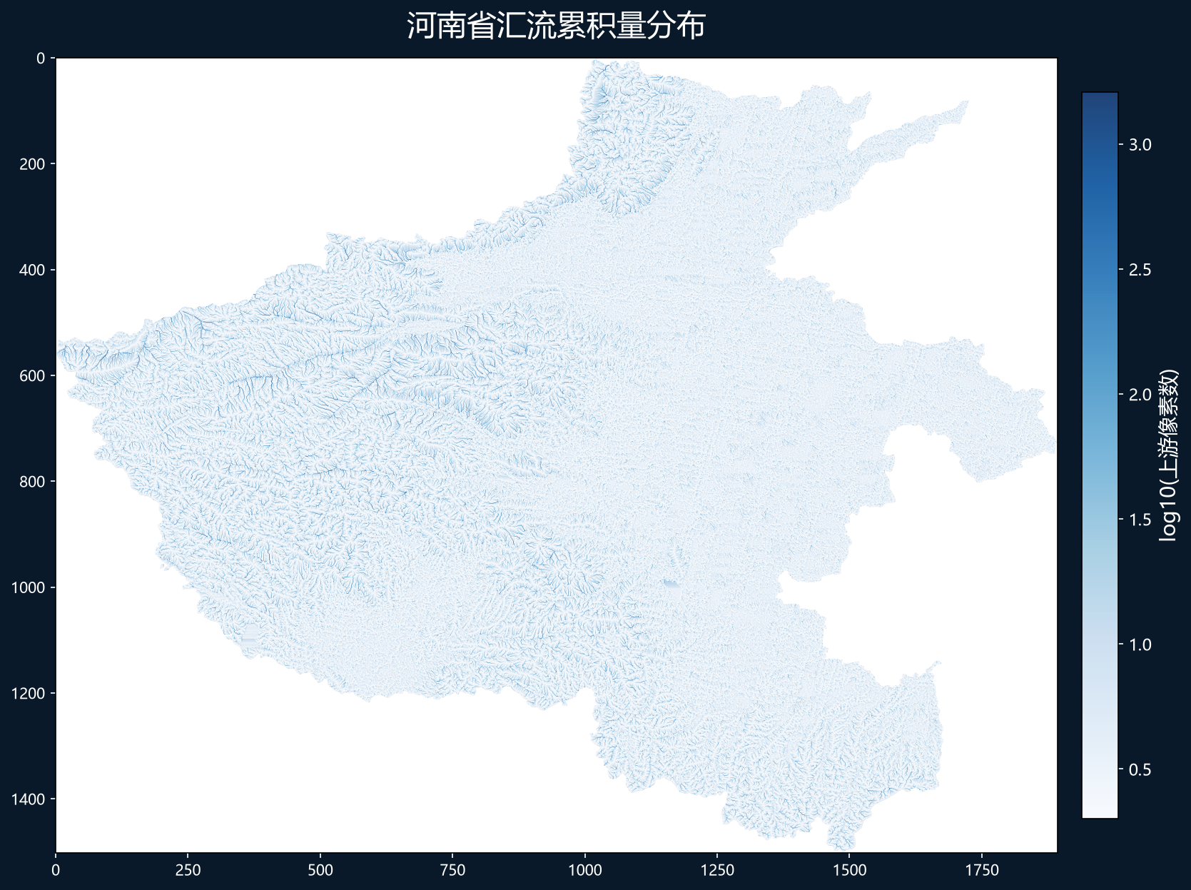
4. 汇流累积(Flow Accumulation)
4.1 原理
沿流向矩阵累加上游来水量。每个像素的汇流累积量等于其自身(1)加上所有流向它的上游像素的汇流累积量之和。
4.2 高效计算
朴素方法是迭代直到收敛(O(n²)),效率低。高效方法:
按高程从高到低对像素排序
依序处理:对每个像素,将自身累积量传递给其下游像素
单次遍历完成(O(n log n))
4.3 河网提取
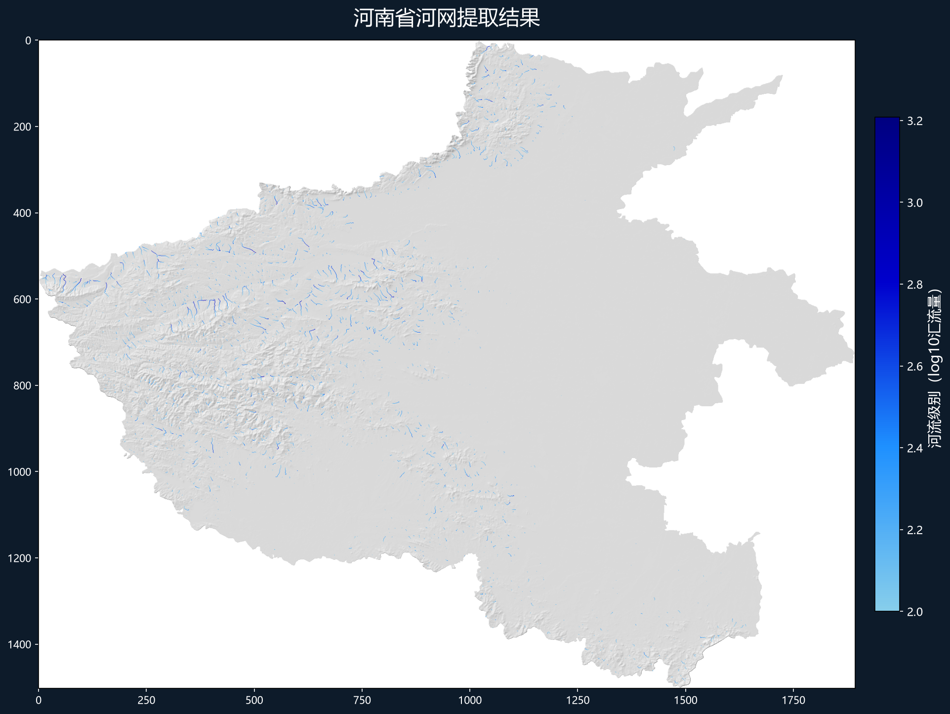
stream = flow_accumulation > threshold
30m GDEM推荐从2000开始,根据目视对比调整。
5. 流域提取(Watershed)
5.1 原理
给定出水口点,沿流向矩阵反向追踪所有上游来源,圈定集水区。
5.2 流域分割
在河流上按等间距布设出水口点,自动分割子流域。这是分布式水文模型(SWAT、HEC-HMS)的空间离散化基础。
# WhiteboxTools: 子流域分割
wbt.strahler_order("streams.tif", "flowdir.tif", "strahler.tif")
wbt.subbasins("flowdir.tif", "streams.tif", "subbasins.tif")
5.3 Strahler河流分级
同级汇合不升级。Strahler级数反映了流域水系发育程度。
6. Python实现
6.1 WhiteboxTools(推荐生产环境)
from whitebox import WhiteboxTools
from pathlib import Path

def hydro_pipeline(dem_path, out_dir, threshold=2000,
                   outlets=None):
    """DEM水文分析完整流程"""
    wbt = WhiteboxTools()
    wbt.set_workdir(str(out_dir))
    stem = Path(dem_path).stem

    # Step 1: 填洼
    print("Step 1/5: 填洼...")
    wbt.fill_depressions(
        dem_path, f"{stem}_filled.tif",
        max_depth=50.0
    )

    # Step 2: D8流向
    print("Step 2/5: 流向(D8)...")
    wbt.d8_pointer(
        f"{stem}_filled.tif",
        f"{stem}_fdir.tif",
        esri_pntr=False  # Whitebox编码(非ESRI)
    )

    # Step 3: 汇流累积
    print("Step 3/5: 汇流累积...")
    wbt.d8_flow_acc(
        f"{stem}_fdir.tif",
        f"{stem}_facc.tif",
        pntr=True  # 输入是D8指针格式
    )

    # Step 4: 河网提取
    print("Step 4/5: 河网提取...")
    wbt.extract_streams(
        f"{stem}_facc.tif",
        f"{stem}_fdir.tif",
        f"{stem}_streams.tif",
        threshold=threshold
    )

    # Step 5: 流域(可选)
    if outlets:
        print("Step 5/5: 流域提取...")
        # 先做河段细微化(snapping)
        wbt.jenson_snap_pour_points(
            outlets, f"{stem}_facc.tif",
            f"{stem}_snap.shp", snap_dist=50.0
        )
        wbt.watershed(
            f"{stem}_fdir.tif",
            f"{stem}_snap.shp",
            f"{stem}_watershed.tif"
        )

    print(f"完成! 输出: {out_dir}")


# 批量处理
if __name__ == '__main__':
    provinces = [
        '110000', '120000', '130000', '140000', '150000',
        '210000', '220000', '230000', '310000', '320000',
        # ... 34省
    ]
    for code in provinces:
        dem = f"/mnt/d/GISData/DEM_V3/a_output/{code}.tif"
        out = f"/mnt/d/GISData/DEM_V3/hydro/{code}"
        Path(out).mkdir(parents=True, exist_ok=True)
        hydro_pipeline(dem, out, threshold=2000)
6.2 GRASS GIS(适合大规模处理)
# 启动GRASS并创建location
grass -c EPSG:4326 ./grassdata/hydro

# 在GRASS命令行中
r.in.gdal input=dem.tif output=dem
r.fill.dir input=dem output=filled areas=problem_areas
r.watershed elev=filled accum=flowacc drain=flowdir \
    threshold=2000 stream=streams basin=watershed
r.stream.extract elevation=filled \
    accumulation=flowacc threshold=2000 \
    stream_vector=stream_network direction=flowdir
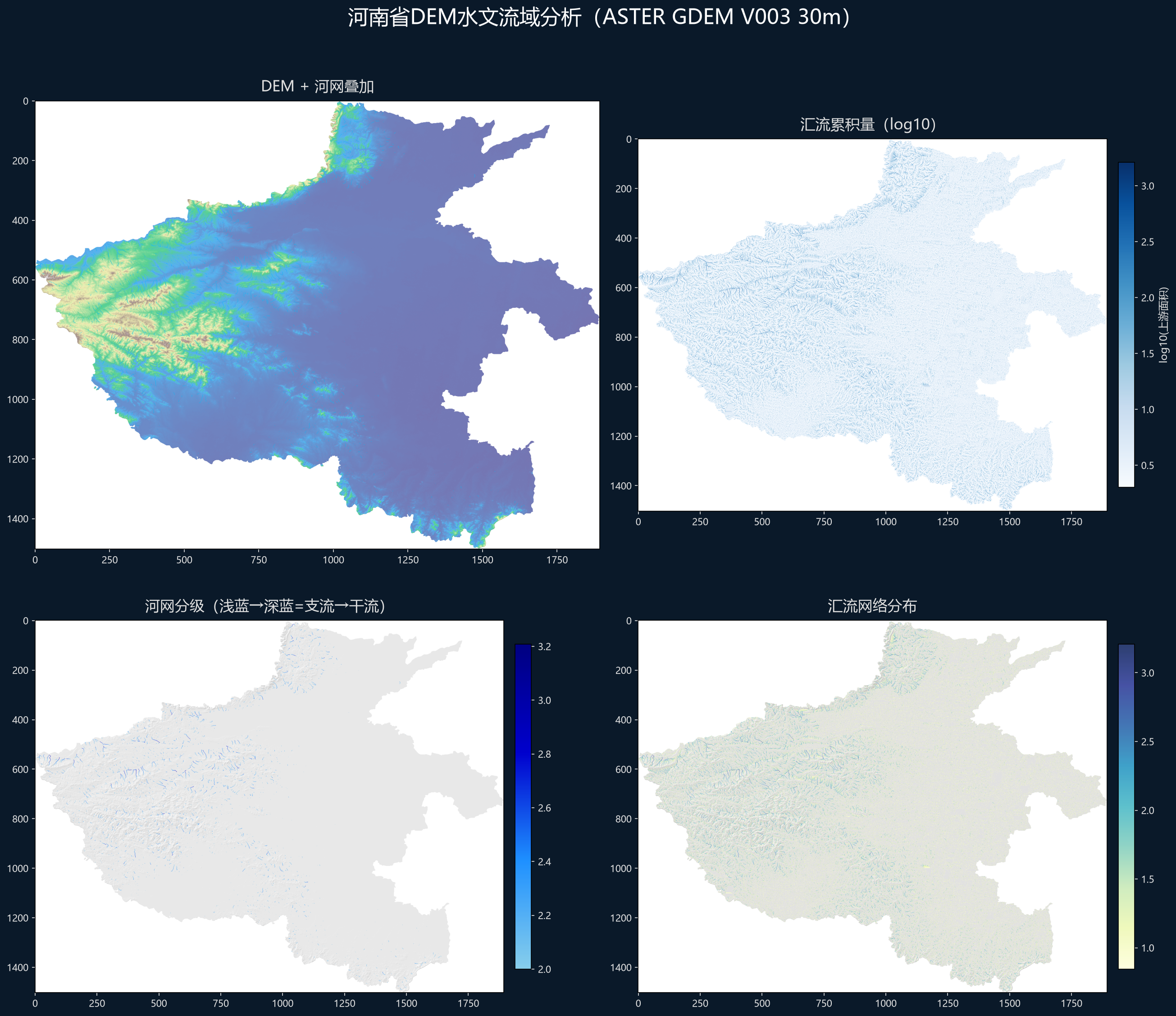
6.3 可视化
import matplotlib.pyplot as plt
import numpy as np
import rasterio
from matplotlib.colors import LogNorm

def plot_hydro_results(base_dir, stem):
    """四合一水文分析可视化"""
    fig, axes = plt.subplots(2, 2, figsize=(16, 14))

    # (1) 填洼后DEM
    with rasterio.open(f"{base_dir}/{stem}_filled.tif") as src:
        dem = src.read(1).astype(float)
        dem[dem == src.nodata] = np.nan
    ax = axes[0, 0]
    ax.imshow(dem, cmap='terrain')
    ax.set_title('填洼后DEM', fontsize=14, fontweight='bold')

    # (2) 汇流累积(对数色标)
    with rasterio.open(f"{base_dir}/{stem}_facc.tif") as src:
        facc = src.read(1).astype(float)
        facc[facc <= 0] = np.nan
    ax = axes[0, 1]
    im = ax.imshow(facc, cmap='Blues', norm=LogNorm(vmin=1, vmax=facc.max()))
    ax.set_title('汇流累积量(对数色标)', fontsize=14, fontweight='bold')
    plt.colorbar(im, ax=ax, shrink=0.7)

    # (3) 河网
    with rasterio.open(f"{base_dir}/{stem}_streams.tif") as src:
        streams = src.read(1)
    ax = axes[1, 0]
    ax.imshow(streams, cmap='gray_r')
    ax.set_title('河网', fontsize=14, fontweight='bold')

    # (4) 流域(如有)
    watershed_path = f"{base_dir}/{stem}_watershed.tif"
    try:
        with rasterio.open(watershed_path) as src:
            ws = src.read(1).astype(float)
            ws[ws <= 0] = np.nan
        ax = axes[1, 1]
        ax.imshow(ws, cmap='tab20')
        ax.set_title('流域', fontsize=14, fontweight='bold')
    except:
        axes[1, 1].set_title('流域(未计算)')

    plt.suptitle('DEM水文分析', fontsize=18, fontweight='bold')
    plt.tight_layout()
    plt.savefig(f'{stem}_hydro.png', dpi=150, bbox_inches='tight')
7. 工具对照
WhiteboxTools是开源免费工具,功能全面且性能优秀,是替代ArcGIS Hydrology工具集的最佳选择。
8. 应用场景
8.1 水库选址
在潜在坝址设定出水口 → 提取流域面积 → 结合降雨估算来水量 → 填洼DEM计算不同水位的库容曲线。
8.2 防洪调度
流域是洪水模拟的空间单元。结合SWAT/HEC-HMS模拟不同降雨条件下的产汇流过程,输出流量过程线用于水库调度。
8.3 引水式电站
山区小型电站选址:提取流域 → 确定引水面积 → 估算发电水头和流量。
8.4 水生态
面源污染(农业化肥、城市径流)按流域追踪。流域是水环境承载力和污染物总量控制的基本空间单元。
8.5 数字孪生流域
水利部正在推进的数字孪生工程,底层数据链就是从DEM→水文分析→流域模型→水动力学模型。DEM水文分析是整个数字孪生流域建设的"第一公里"。
9. 数据获取
本文分析基于 ASTER GDEM V003(30m精度),全国34省已处理裁切完毕。
方式一:公众号私信
关注公众号「YouGIS顽石」,发送关键词:
方式二:YouGIS数据助手
微信小程序:搜索「YouGIS数据助手」
参考文献
Jenson, S.K. & Domingue, J.O. (1988). Extracting topographic structure from digital elevation data for geographic information system analysis. PE&RS, 54(11):1593-1600.
O’Callaghan, J.F. & Mark, D.M. (1984). The extraction of drainage networks from digital elevation data. CVGIP, 28(3):323-344.
Tarboton, D.G. (1997). A new method for the determination of flow directions and upslope areas in grid DEMs. WRR, 33(2):309-319.
Planchon, O. & Darboux, F. (2001). A fast, simple and versatile algorithm to fill the depressions of DEMs. Catena, 46(2-3):159-176.
Lindsay, J.B. (2016). Efficient hybrid breaching-filling sink removal methods for flow path enforcement in DEMs. Hydrological Processes, 30(6):846-857.
数据来源:ASTER GDEM V003(NASA/METI),YouGIS顽石整理加工与分享。
评论区