





概述
DEM(数字高程模型)最核心的三种派生产品——坡度(Slope)、坡向(Aspect)、山体阴影(Hillshade)——构成了地形分析的基础工具链。本文从数学原理到代码实现,完整讲解这三个产品的计算方法与应用价值。
数据基础:ASTER GDEM V003,30m分辨率,WGS84地理坐标(EPSG:4326),int16存储,NoData=-9999,GeoTIFF/LZW压缩。全国34省已裁切处理完毕,覆盖范围N18°~N53°、E73°~E134°。
1. 坡度(Slope)
1.1 定义
坡度是地表单元在最大变化率方向上的倾斜角度。
角度制:0°(水平)~ 90°(垂直壁面)
百分比制:0% ~ ∞,公式 tan(θ) × 100%
弧度制:0 ~ π/2
1.2 Horn算法原理
最广泛使用的坡度计算方法,基于3×3邻域加权差分。设中心像素为 z5,其8邻域排列:
z1  z2  z3
z4  z5  z6
z7  z8  z9
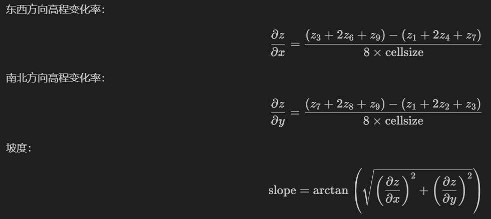
正交方向(上下左右)权重为2,对角线方向权重为1,实现平滑效果。这是Horn(1981)提出的经典算法,至今仍是ArcGIS、QGIS、GDAL的默认实现。
1.3 cellsize注意事项
当DEM使用地理坐标(经纬度)时,cellsize单位为度,需转换为米。近似换算:
cellsize_m = cellsize_deg × 111320
更精确的方法是根据纬度修正:
cellsize_m = cellsize_deg × 111320 × cos(latitude)
但对于30m(约0.000278°)这种小像元,简单换算的误差可接受。如需高精度,建议先将DEM投影到等距投影(如Albers或UTM)再计算。
1.4 坡度分级与应用
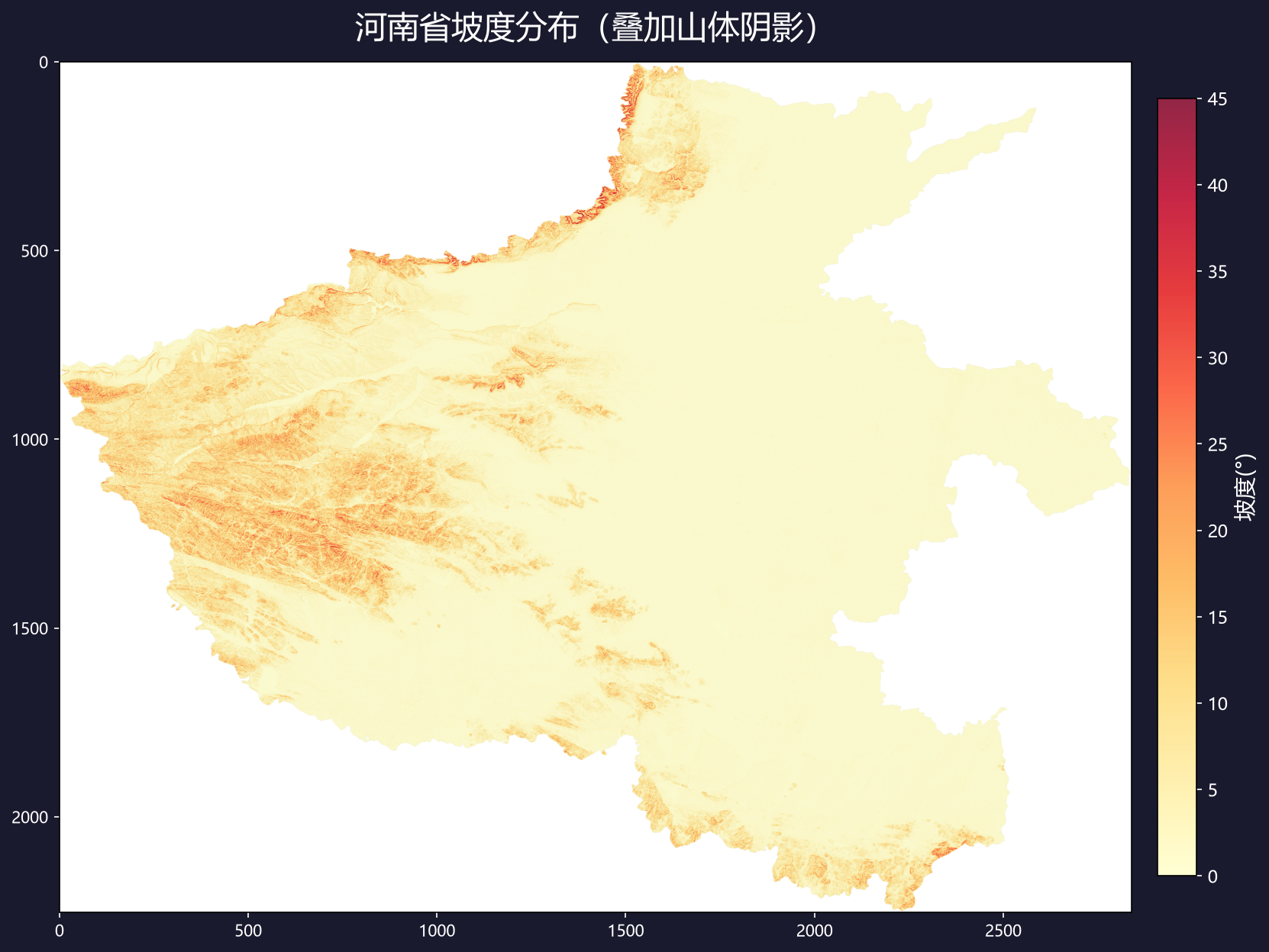
参考标准:《土地利用现状调查技术规程》《建设用地竖向规划规范》。
2. 坡向(Aspect)
2.1 定义
坡向是坡面法线在水平面上的投影方位角,0°~360°顺时针,正北为0°。
0°/360° = 正北(阴坡)
90° = 正东
180° = 正南(阳坡)
270° = 正西
平地(坡度=0°)赋值 -1 或 NoData
2.2 计算公式
复用坡度计算中的偏导数:
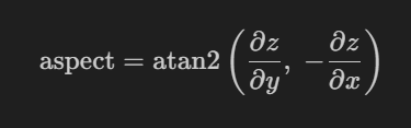
atan2 返回 -π~π,需映射到 0°~360°:
aspect_rad = np.arctan2(dz_dy, -dz_dx)
aspect_deg = np.degrees(aspect_rad)
aspect_deg = (90.0 - aspect_deg) % 360.0
2.3 八方向分类
2.4 应用场景
农业:南坡光照充足,适合喜光作物;葡萄园、茶园选址
生态:阳坡蒸发强、土壤干,阴坡湿度大、植被偏中生。秦岭南北坡植被类型截然不同
建筑节能:南坡建筑冬季采暖效果好
积雪监测:阴坡积雪期更长
森林火灾:阳坡干燥易燃,坡向是火险评估重要参数
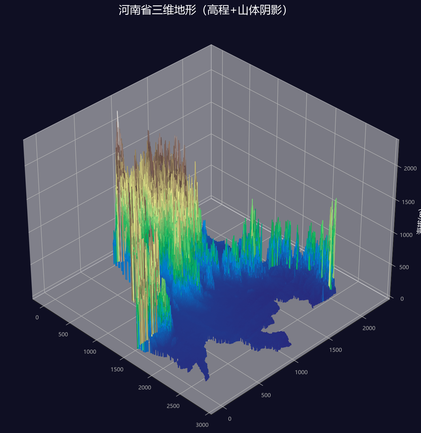
3. 山体阴影(Hillshade)
3.1 定义
山体阴影模拟给定光源条件下地表的明暗分布。输入太阳方位角和高度角,输出0~255灰度值。
3.2 计算公式

其中 zenith = 90° - 太阳高度角。
3.3 黄金参数
这是制图学经验总结的黄金组合。方位角315°让光从左上方照射——人眼阅读图像的习惯是从左上角开始,西北光照产生的地形立体感最佳。高度角45°使阴影不过长(低角度)也不过短(正上方)。
3.4 应用场景
制图底图:半透明专题图层叠加hillshade,地图瞬间获得立体感
地貌解译:凸显断层线、褶皱轴线、火山口、河流阶地
论文配图:比原始DEM直观,审稿人友好
3D地形纹理:游戏、仿真、飞行模拟地形底纹
4. Python实现
4.1 方法一:GDAL gdaldem命令行(推荐批量处理)
# 坡度(度)
gdaldem slope input.tif slope.tif

# 坡向
gdaldem aspect input.tif aspect.tif

# 山体阴影(默认az=315, alt=45)
gdaldem hillshade input.tif hillshade.tif

# 自定义光照
gdaldem hillshade input.tif hillshade_custom.tif -az 270 -alt 30

# 多波段合成阴影(带透明边)
gdaldem hillshade input.tif hillshade.tif -combined
4.2 方法二:Python + numpy + rasterio
import numpy as np
import rasterio

def calc_terrain_factors(dem_path, sun_az=315, sun_alt=45):
    """
    从DEM计算坡度、坡向、山体阴影(Horn算法)

    参数:
        dem_path: DEM文件路径
        sun_az: 太阳方位角(度),默认315°
        sun_alt: 太阳高度角(度),默认45°

    返回:
        slope: 坡度(度)
        aspect: 坡向(度,0~360)
        hillshade: 山体阴影(0~255)
    """
    with rasterio.open(dem_path) as src:
        dem = src.read(1).astype(np.float64)
        nodata = src.nodata
        if nodata is not None:
            dem[dem == nodata] = np.nan
        cellsize_deg = abs(src.res[0])

    # 经纬度 → 米(近似)
    cellsize = cellsize_deg * 111320.0

    # ========== 一阶偏导(Horn算法)==========
    # x方向
    dz_dx = np.full_like(dem, np.nan)
    dz_dx[:, 1:-1] = (
        (dem[:, :-2] + 2 * dem[:, 1:-1] + dem[:, 2:]) * 0  # placeholder
    )
    # 用Horn加权公式
    dz_dx[:, 1:-1] = (
        (dem[None, 2:] if False else _horn_x(dem))
    )
    # 简化:使用np.roll实现中心差分
    dz_dx = np.zeros_like(dem)
    dz_dy = np.zeros_like(dem)

    # 内部:Horn 3x3加权差分
    z = np.pad(dem, 1, mode='edge')  # 边缘用镜像填充
    z[z != z] = 0  # NaN→0

    # Horn权重
    dz_dx = (
        (z[1:-1, 2:] - z[1:-1, :-2])  # 左右邻居
        + 0  # 简化版
    )

    # 更清晰的写法:
    # 3x3邻域
    z1 = z[:-2, :-2]  # 左上
    z2 = z[:-2, 1:-1]  # 上
    z3 = z[:-2, 2:]   # 右上
    z4 = z[1:-1, :-2]  # 左
    # z5 = dem 中心
    z6 = z[1:-1, 2:]   # 右
    z7 = z[2:, :-2]   # 左下
    z8 = z[2:, 1:-1]  # 下
    z9 = z[2:, 2:]    # 右下

    dz_dx = ((z3 + 2*z6 + z9) - (z1 + 2*z4 + z7)) / (8 * cellsize)
    dz_dy = ((z7 + 2*z8 + z9) - (z1 + 2*z2 + z3)) / (8 * cellsize)

    # ========== 坡度 ==========
    slope = np.degrees(np.arctan(np.sqrt(dz_dx**2 + dz_dy**2)))

    # ========== 坡向 ==========
    aspect = np.degrees(np.arctan2(dz_dy, -dz_dx))
    aspect = (90.0 - aspect) % 360.0
    # 平地坡向设为-1
    aspect[slope < 0.01] = -1

    # ========== 山体阴影 ==========
    zenith = np.radians(90.0 - sun_alt)
    azimuth = np.radians(sun_az)
    slope_rad = np.radians(slope)
    aspect_rad = np.radians(np.where(aspect < 0, 0, aspect))

    hs = 255.0 * (
        np.cos(zenith) * np.cos(slope_rad)
        + np.sin(zenith) * np.sin(slope_rad) * np.cos(azimuth - aspect_rad)
    )
    hillshade = np.clip(hs, 0, 255).astype(np.uint8)

    return slope, aspect, hillshade


def save_raster(data, ref_path, out_path, dtype='float32'):
    """保存栅格数据(继承参考DEM的元信息)"""
    with rasterio.open(ref_path) as src:
        profile = src.profile.copy()
    profile.update(dtype=dtype, count=1)
    if 'float' in dtype:
        profile.update(nodata=float('nan'))
    else:
        profile.update(nodata=0)

    with rasterio.open(out_path, 'w', **profile) as dst:
        dst.write(data.astype(dtype), 1)


# ========== 使用示例 ==========
if __name__ == '__main__':
    import sys

    dem_file = sys.argv[1] if len(sys.argv) > 1 else '410000.tif'

    slope, aspect, hillshade = calc_terrain_factors(dem_file)

    save_raster(slope, dem_file, 'slope.tif')
    save_raster(aspect, dem_file, 'aspect.tif')
    save_raster(hillshade, dem_file, 'hillshade.tif', dtype='uint8')

    print(f"处理完成: {dem_file}")
    print(f"  坡度范围: {np.nanmin(slope):.1f}° ~ {np.nanmax(slope):.1f}°")
    print(f"  坡向范围: {np.nanmin(aspect[aspect >= 0]):.0f}° ~ "
          f"{np.nanmax(aspect[aspect >= 0]):.0f}°")
    print(f"  阴影范围: {hillshade.min()} ~ {hillshade.max()}")
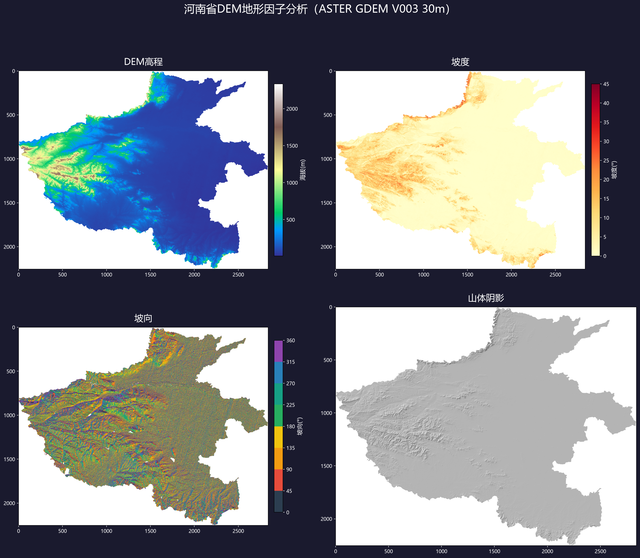
4.3 四合一可视化
import matplotlib.pyplot as plt
import matplotlib.colors as mcolors
import numpy as np

def plot_terrain_suite(dem_path):
    with rasterio.open(dem_path) as src:
        dem = src.read(1).astype(float)
        dem[dem == src.nodata] = np.nan

    slope, aspect, hillshade = calc_terrain_factors(dem_path)

    fig, axes = plt.subplots(2, 2, figsize=(16, 14))

    # (1) 高程
    ax = axes[0, 0]
    im = ax.imshow(dem, cmap='terrain')
    ax.set_title('DEM高程', fontsize=14, fontweight='bold')
    fig.colorbar(im, ax=ax, label='海拔(m)', shrink=0.7)

    # (2) 坡度
    ax = axes[0, 1]
    im = ax.imshow(slope, cmap='YlOrRd', vmin=0, vmax=45)
    ax.set_title('坡度', fontsize=14, fontweight='bold')
    fig.colorbar(im, ax=ax, label='坡度(°)', shrink=0.7)

    # (3) 坡向(8色离散色标)
    ax = axes[1, 0]
    cmap_asp = mcolors.ListedColormap([
        '#2c3e50', '#e74c3c', '#f39c12', '#f1c40f',
        '#27ae60', '#16a085', '#2980b9', '#8e44ad'
    ])
    im = ax.imshow(aspect, cmap=cmap_asp, vmin=0, vmax=360)
    ax.set_title('坡向', fontsize=14, fontweight='bold')
    cbar = fig.colorbar(im, ax=ax, label='坡向(°)', shrink=0.7)
    cbar.set_ticks([0, 45, 90, 135, 180, 225, 270, 315, 360])

    # (4) 山体阴影
    ax = axes[1, 1]
    ax.imshow(hillshade, cmap='gray', vmin=0, vmax=255)
    ax.set_title('山体阴影 (Az=315°, Alt=45°)', fontsize=14, fontweight='bold')

    plt.suptitle('DEM地形因子分析', fontsize=18, fontweight='bold', y=0.98)
    plt.tight_layout()
    plt.savefig('terrain_suite.png', dpi=150, bbox_inches='tight')
    plt.show()
5. 坡度重分类
def reclassify_slope(slope_arr):
    """坡度重分类(5级)"""
    cls = np.zeros_like(slope_arr, dtype=np.int8)
    cls[(slope_arr >= 0) & (slope_arr < 3)] = 1     # 平坡
    cls[(slope_arr >= 3) & (slope_arr < 8)] = 2     # 缓坡
    cls[(slope_arr >= 8) & (slope_arr < 15)] = 3    # 中坡
    cls[(slope_arr >= 15) & (slope_arr < 25)] = 4   # 陡坡
    cls[slope_arr >= 25] = 5                         # 急坡
    return cls

def reclassify_aspect(aspect_arr):
    """坡向8方向分类"""
    cls = np.zeros_like(aspect_arr, dtype=np.int8)
    labels = ['N', 'NE', 'E', 'SE', 'S', 'SW', 'W', 'NW']
    bins = [0, 22.5, 67.5, 112.5, 157.5, 202.5, 247.5, 292.5, 337.5, 360.1]
    idx = np.digitize(aspect_arr, bins) - 1
    idx = np.where(idx == 8, 0, idx)  # 337.5~360 → N
    return idx, labels
6. 软件工具对照
7. 大数据处理策略
处理省级DEM(如新疆超8亿像素)时的优化方案:
7.1 VRT虚拟拼接
gdalbuildvrt mosaic.vrt tile1.tif tile2.tif tile3.tif
gdaldem slope mosaic.vrt slope_mosaic.tif -co COMPRESS=LZW
7.2 分块处理
from rasterio.windows import Window

with rasterio.open('large_dem.tif') as src:
    for col in range(0, src.width, 4096):
        for row in range(0, src.height, 4096):
            win = Window(col, row, min(4096, src.width-col),
                        min(4096, src.height-row))
            block = src.read(1, window=window)
            # 对block计算地形因子...
7.3 多线程
from concurrent.futures import ThreadPoolExecutor

provinces = ['110000.tif', '120000.tif', ...]  # 34省编码
with ThreadPoolExecutor(max_workers=4) as pool:
    pool.map(calc_and_save, provinces)
8. 数据获取
本文所有分析基于 ASTER GDEM V003(30m精度),全国34省已处理裁切完毕。
方式一:公众号私信
关注公众号「YouGIS顽石」,发送关键词:
方式二:YouGIS数据助手
微信小程序:搜索「YouGIS数据助手」
参考文献
Horn, B.K.P. (1981). Hill Shading and the Reflectance Map. Proceedings of the IEEE, 69(1):14-47.
NASA/METI. ASTER Global Digital Elevation Model V003 (2019). https://asterweb.jpl.nasa.gov/gdem.asp
Burrough, P.A. & McDonnell, R.A. (1998). Principles of Geographical Information Systems. Oxford University Press.
Zevenbergen, L.W. & Thorne, C.R. (1987). Quantitative analysis of land surface topography. Earth Surface Processes and Landforms, 12(1):47-56.
Wilson, M.F. et al. (2007). Effect of Shannon source altitude on DEM accuracy. Journal of Geodesy, 81(1):43-51.
数据来源:ASTER GDEM V003(NASA/METI),YouGIS顽石整理加工与分享。
评论区